The purpose of the following activity was to familiarize ourselves with the different functions and processing techniques in scilab. In this activity, various images that are useful in image processing were synthesized.
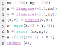
The first image produced was a circular aperture. A 2D array was created with elements valued by its distance from the center. By setting a threshold value (r<0.7) these values were then set to 1 in a zero array. The code and results are shown below:
The second image to be produced was a square aperture. The synthesis of this image was done similar to the above image, except instead of radial values, x and y values were processed separately such that one end of the zero array was changed into ones and then the edge of that was changed back into zeros. The results produced the following image:
The next image synthesized was a sinusoid in the x-direction. Similar to the previous codes, it starts with a 2D array. The values of the 2D array were changed such that the values changed sinusoidally in the x-direction.
The next image, a grating, is extremely similar to producing the sinusoid in the x direction. In order to remove the gradient to produce a sharp grating, a threshold was set such that values above it are changed to 1 and values below are changed to zero. The result is the image below:
Creating the next image, an annulus, is done by simply adding another line of code to the code for the circular aperture, setting another threshold such that values below the threshold are zero again.
The final image is a circular aperture with graded transparency (gaussian). For this particular image, we simply make use of the function fspecial(). By inputting the parameters ‘gaussian’, size and sigma value, the function automatically generates a 2D array with values that follow a gaussian curve.
One particular error I encountered while manipulating the code was an error with the available stack space. At the start, the error, which stated that I had insufficient space for my variables, limited me to smaller images. The command stacksize(‘max’) ordinarily resolves this problem, but this was not the case for me. In order to resolve this, I had to manually reset the stack size to a specific value 1e8, instead of the default ‘max’.
The activity’s purpose is to be able to process the data from an analog or hand-drawn graph by scanning the figure and processing the values digitally.
Shown below is the graph to be processed from J. Opt. Soc. Vol. 2, No. 11, November 1985 by Michael Teague on image formation in terms of the transport equation:
Given a digitally scanned image, all points in the image can now be defined by the location of certain pixels. The coordinates of the lower-left corner of the image are taken, and replotted on excel as (0,0). In this particular image, where the pixels are counted form the upper-left corner, the coordinates for the new origin were at (112,380).
After establishing the new origin point, other key information is taken from the image using the coordinates of the pixels. One of the values obtained was the number of pixels between each tick on the x and y axis. These values were 31 pixels and 37 pixels respectively and knowing these will help in scaling the processed data.
Also obtained were certain points on the line graph. In this case, I took the coordinates of the maxima and minima shown. Since the pixel coordinates are taken with the origin of the upper-left, an equation in excel made it such that the two coordinates were arranged on the positive x and positive y axis. The values were then shifted by subtraction (so that the central maximum was at zero) and the values were scaled (so that the maximum value was 100000).
Once this has all been plotted in excel and been scaled appropriately, we can interpolate for the other values. We can also check the accuracy of the digital scanning by overlaying the original image on the created graph as shown below.
Although the interpolated data has a slight deviation from the original image, particularly in the central maxima, the data is accurate to some extent. The reason for the error may be due to the fact that the original image was slightly skewed, giving inaccurate values for the pixel coordinates. For this reason, I will be giving myself a grade of 8/10 for this activity.
Welcome to WordPress.com! This is your very first post. Click the Edit link to modify or delete it, or start a new post. If you like, use this post to tell readers why you started this blog and what you plan to do with it.
Happy blogging!


