Histogram Manipulation

The objective of the activity we are about to discuss is to manipulate an image through the values of its histogram. As we already know, pixels in grayscale images are assigned levels from 0-255, with 0 being the darkest and 255 being the lightest. Calling a completely white image would give us an 2D array of 255s while a black image would give us an array of zeros.

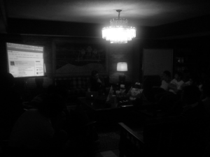
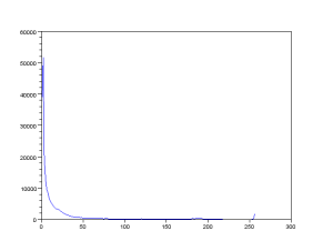
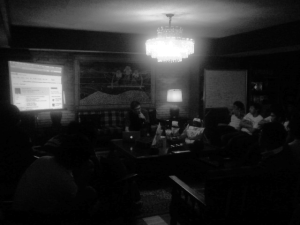
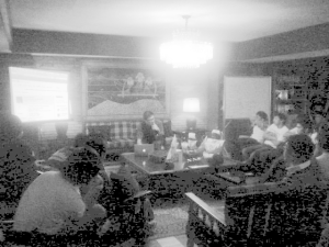
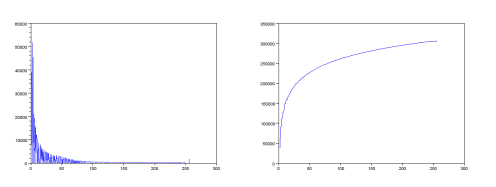
The manipulation of the image is primarily concerned with the histogram of the gray values in an image. Say that a picture is taken in the dark. The result would be that most of the pixels in the image would be assigned lower values, which would be made apparent in the image’s histogram. Below is an example of a dark grayscale image and its point distribution function from its histogram.

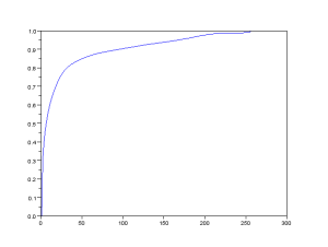
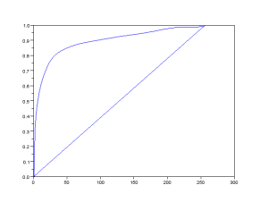
As we can see from the images, the number of counts on the histogram are higher on the left end of the axis, meaning there are more pixels with lower values. We take the values from the histogram and arrange it as a cumulative sum. This gives us the cumulative distribution function(CDF) of the image.

We now decide for a shape for our desired CDF. We want to improve the image by shifting the darker pixels to lighter ones, but we do not want to shift them too far or this will result in different levels crowding into a single gray level, particularly at higher values. We also want the shift to be proportionate to their original values. These requirements help to pick an appropriate shape for the CDF.

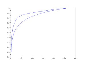
Since the image CDF looks like a logarithmic function, we plot our ideal CDF as a logarithmic function with a lower incline.

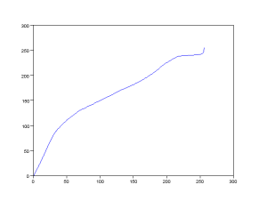
Now that we have our original CDF and ideal CDF, we need to create a translator saying that all pixels with x1 gray level will then be changed to x2 gray level. We do this by backplotting, that for every x-value in the original CDF, we look at its y-value, find the closest existing y-value in the ideal CDF and take the x-value. This was done by assigning the y-value of the original CDF to a variable. Using the find function, I located the indices for which the y-value was greater and the indices the y-value was smaller. I would then simply compare if the last of the smaller values or the first of the greater values to see which was closer to the y-value. Whichever was closer would be the corresponding point. Below is an example of the plot of the resulting translator.

Translator for the logarithmic function

The plots above show the translation from x1 to x2. A straight slope means no change, a high slope means a shift to higher values, and a low slope means a shift to lower values. We simply apply this translator to the image and we have our final result.

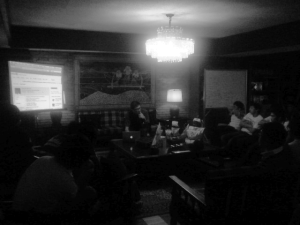
The two images above are created using two different logarithmic CDFs, with different slopes. The more we slope the ideal CDF away from the original CDF, the lighter the image becomes. However, this results in the higher values crowding the remaining gray levels, resulting in quantization error. This is apparent in the lighter areas of the image.

Suppose we chose an ill-fitting CDF for the histogram manipulation, the result would end up translating pixels to disproportionate levels, resulting in an increased occurrence of quantization errors. The images below show a linear CDF, its translator and the results.

Original CDF and ideal CDF

Translator from the CDF

Result from linear ideal CDF.

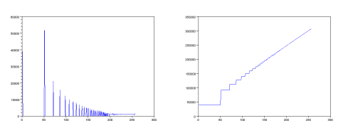
Having successfully manipulated the histogram of the image, we want to look at the new PDF and CDF of the image. Below are some examples.

Logarithmic CDF applied

Linear CDF applied

We can see from the above images that histogram of the image has changed such that there are now numerous values with zeros, resulting in a plot with a jagged appearance. We also note that the CDF attempts to imitate the applied ideal CDF. Both are the effects of quantization error.

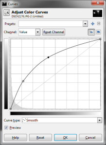
We also perform histogram manipulation on the same image using GIMP 2.8. Using the same shape CDF on the image, we achieve a similar result as shown below.

Having achieved the results of the activity, and giving a sufficient discussion on implementing the histogram manipulation technique, I will give myself a grade of 11/10 for this exercise.