Image Types and Formats

Digital images can come in many different forms based on the properties of the image, on how the data is stored or represented, or how the image is used.

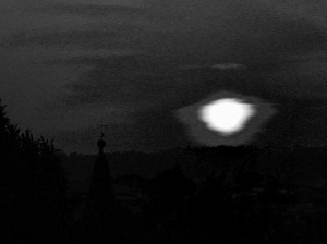
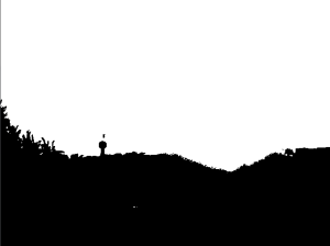
The most basic image type is the binary image. The entire image is simply composed of 1s and 0s, creating a pure black and white image with no graylevels. It is a very compact way of representing an image since the data is represented so simply. Below is an example of a binary image:

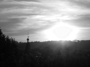
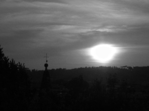
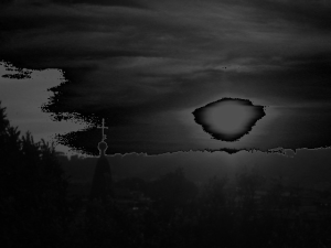
Another image type is the grayscale image. Similar to the binary image, it also shows images with black and white, however, italso allows variation between black (represented as 0) and white (represented as 255), allowing varying levels of gray in between. Below is an example of a grayscale image.

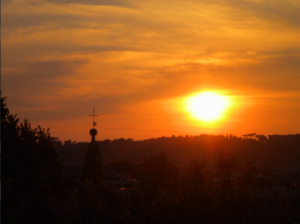
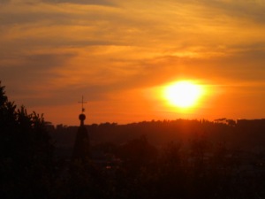
Truecolor images are able to display images in full color by representing each color with values for red, green, and blue for each pixel. The result is a 3d image, or rather, a 3-layered 2d image, each layer containing values for red, green, and blue. This image type allows for large color variation, at the cost of increased file size.

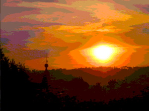
Indexed color images, like the truecolor images, are able to represent color images. However, instead of having a 3-layered image with each layer for red, green, and blue, Each pixel is represented with a value which corresponds to the index of a particular color. The result is an image that requires less space, but has less flexibility in color representation, as shown below.

The above four are the basic image types. However, besides, them, there are other image types, such as High dynamic range images, which have greater bitdepth, multi- or hyperspectral images, which have color representations other than the usual red, green, and blue, 3D images and videos. For the HDR images and the hyperspectral images, I am unable to open and edit such files on my laptop without the proper programs.

While the data that images can provide are important, it is also important to know what information within the image is important. For image processing techniques that require only a general trend, a simple black and white image file can suffice. For others, it may require the use of different gray levels, or even the use of colors. Depending on the purpose of the image, it may be more effective to use different file types.

Below is a list of the more common file types and some of their properties:

1. .bmp (bitmap) – used primarily in Windows applications. It may contain different levels of color depth depending on the specified bit per pixel.
2. .jpg – a compressed image format commonly used for storing digital photos. It supports 24-bit color, making it the default image type for cameras. Depending on the compression used, the lossy file type can severely reduce the quality of the image.
3. .gif – contains 256 indices for colors, which can be predefined or set to match the colors of an image. It is a lossless file type, so no data is lost. It can also be used to show ‘animations’, but are unsuitable for photos due to the limited color index. Also has copyright issues.
4. .png – similar to GIF such that is uses indexed colors and is a lossless file type. Unlike the GIF, it cannot support animations, but it does have an 8-bit transparency channel for transparent or opaque colors.
5. .tif – can be used for images with many colors, and can be set as lossy or lossless. It can also utilize LZW  compression which reduces the file size but does not compromise the quality.

We move on to doing some simple image processing techniques using scilab. I’ve taken a truecolor image for our purposes as shown below.

Using scilab to determine its properties, I’ve found that the image size is 480 x 640x 3, a 3d array. The first 2 dimensions are for the xy-coordinates we see. The third dimension is for the depth of color for red, green, and blue. If we were to call each color seperately, the following would appear:

red filter

green filter

blue filter

We note that the images are shown in grayscale instead of their actual color shades of red, green, and blue. This is because within the 3d matrix, these values are only recorded in values from 0-255, identical to the format of a grayscale image. Therefore, darker spots on the image would mean lower values for that particular color and lighter areas would mean high values. Since the original image was predominantly red and yellow, it makes sense that the color with the darkest image is the blue filtered image. We confirm this by taking  the histogram of the blue filter:

histogram of blue intensities

As we can see from the histogram, the pixels with low blue values are more than those with high blue values, indicating that the image has very little blue, supporting what we know of the original image.

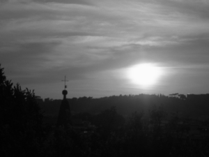
We then move on to converting the true color image into gray scale. Since the original image contains information for values of red, green, and blue, it inevitably takes up more space when color may not be necessary. By converting it to grayscale, we get an image that  has only one plane of information. Below is the grayscale of the original true color image:

grayscale image

Taking the size of the grayscale image, we find that it has been reduced to a 2d image: 480 x 640 pixels. Comparing the values of the grayscale image to the original truecolor image, the grayscale image is at the very least, not the average of the values of red, green, and blue. The average of the three colors put together would produce the following image:

This is clearly not a good representation of the original image. Whatever the method, scilab was able to create an accurate representation of the original image with less data.

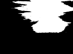
From the grayscale image, we create a binary image of the original picture. We can set the threshold value to different levels from 0-1, selecting the dividing point of which will be changed to 0s and which will be changed to 1s. Below is the resulting binary image with different threshold values.

Threshold at 0.2

Threshold at 0.5

 Threshold at 0.8

Changing an image to binary is very useful when cleaning images such as graphs. The data provided by graphs in general should be binary, but at times, some unnecessary data appears during the capturing of the image. For example, the graph we used in the previous activity, by looking at the information, is a true color image.

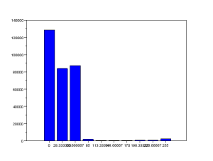
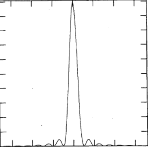
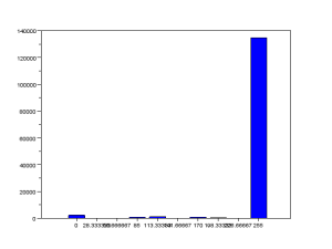
If we were to view the image closely, there are various points on the line graph that are somewhat fainter than the rest of the line. This could lead to reading the data inaccurately. We take the histogram of the image to see what are the values across the image.

The image is predominantly white, so we expect the high count on the far end of the histogram. We want to change this image into binary so that the ambiguous gray pixels are replaces with either white or black. We choose a point that includes the three smaller values on the histogram. The resulting image is

The result is a much clearer image. One should be careful in choosing the threshold value. Too high and noise becomes more prominent. Too low and data is lost. We can then simply save this new image into the appropriate filetype using the function imwrite().

For this activity, I give myself a 10/10. Although the examples for the various image types are somewhat lacking, I believe I was able to make up for it with the extent I investigated and manipulated the images using scilab.